1. Introduction
2. Configuration Class
class CFG:
    # Model weights
    lgb_weight = 0.20
    ctb_weight = 0.20
    xgb_weight = 0.20
    ridge_weight = 0.20
    rfr_weight = 0.20

    # Parameters for models
    lgb_params = {
        'objective': 'regression',
        'learning_rate': 0.03,
        'num_iterations': 4000,
        'max_depth': 4,
        'seed': 42
    }
    ctb_params = {
        'loss_function': 'RMSE',
        'learning_rate': 0.03,
        'num_trees': 4000,
        'depth': 4,
        'random_state': 42
    }
    xgb_params = {
        'objective': 'reg:squarederror',
        'learning_rate': 0.03,
        'max_depth': 4,
        'n_estimators': 4000,
        'seed': 42
    }
    ridge_params = {
        'alpha': 1.0,
        'solver': 'auto',
        'random_state': 42
    }
    rfr_params = {
        'n_estimators': 1000,
        'max_depth': 10,
        'random_state': 42
    }
3. Defining Numerical and Categorical Columns
4. Outlier Detection and Removal
- Visualization: Plotted numeric features against the target variable (SalePrice) to visually inspect relationships and identify potential outliers.
- Z-score Method: Removed outliers from selected numeric features using a Z-score threshold of 4.5.
# Step 1: Visualization
# Define the target column and select numeric features only, excluding the target
target_column = 'SalePrice'
feature_columns = [col for col in numeric_cols if col != target_column]

# Determine the number of rows needed for a 4-column layout
num_columns = 4
num_rows = ceil(len(feature_columns) / num_columns)

# Set up the figure and axes
fig, axes = plt.subplots(num_rows, num_columns, figsize=(20, num_rows * 5), facecolor=CFG.background_color)
fig.subplots_adjust(hspace=0.4, wspace=0.4)

# Flatten the axes array for easy iteration
axes = axes.flatten()

# Plot each feature against SalePrice
for i, feature in enumerate(feature_columns):
    ax = axes[i]
    ax.set_facecolor(CFG.background_color)  # Set background color of each plot
    ax.scatter(CFG.train_df[feature], CFG.train_df[target_column], s=5, color=CFG.point_color)
    ax.set_title(feature, color=CFG.font_color)  # Title is now only the feature name
    ax.set_xlabel('')  # Remove x-axis label name only
    for spine in ax.spines.values():  # Remove the border
        spine.set_visible(False)
    ax.tick_params(axis='x', colors=CFG.font_color)  # Apply font color to tick labels
    ax.tick_params(axis='y', colors=CFG.font_color, labelleft=False)

# Hide any unused axes if the number of plots is less than the grid
for j in range(i + 1, len(axes)):
    fig.delaxes(axes[j])

plt.show()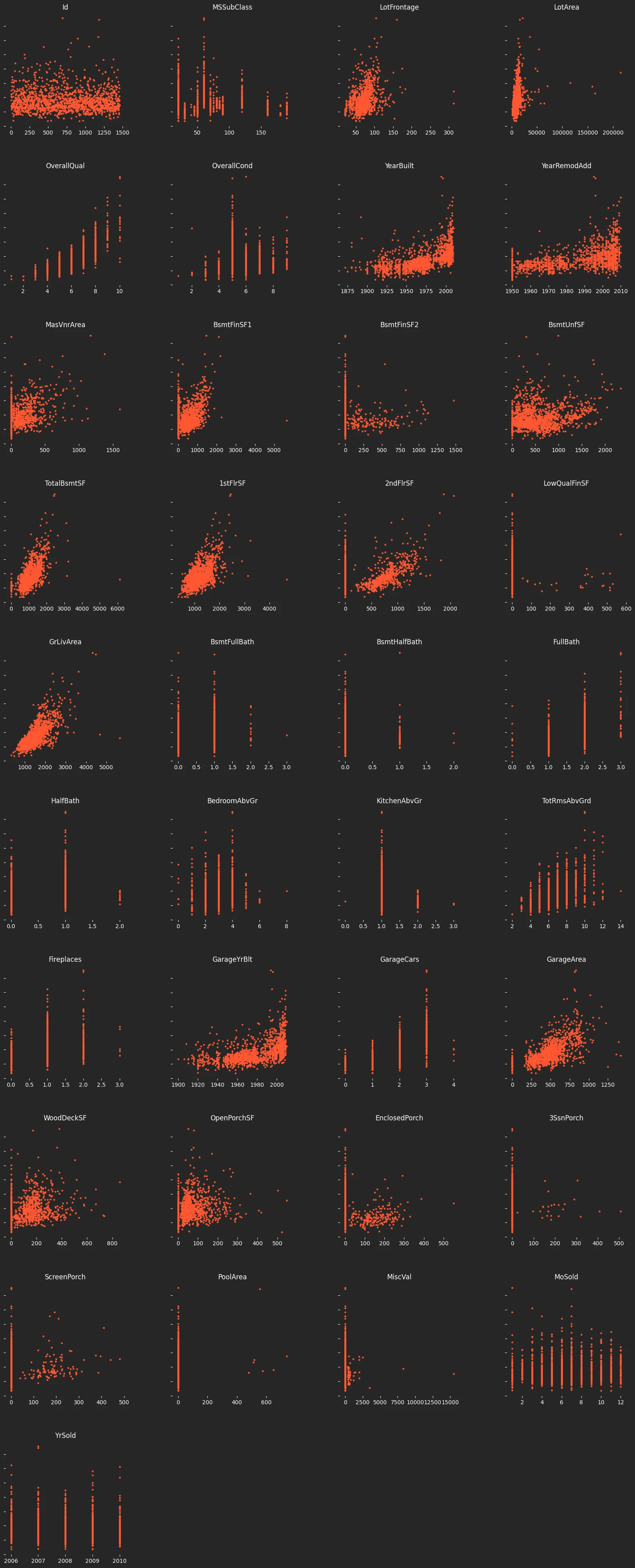
# Step 2: Outlier Removal
# Define columns with and without outliers
without_outliers = [
    'Id', 'MSSubClass', 'OverallQual', 'OverallCond', 'YearBuilt',
    'YearRemodAdd', 'BsmtUnfSF', 'LowQualFinSF', 'BsmtFullBath',
    'BsmtHalfBath', 'FullBath', 'HalfBath', 'TotRmsAbvGrd',
    'Fireplaces', 'GarageYrBlt', 'GarageCars', 'GarageArea',
    'MoSold', 'YrSold'
]
with_outliers = [col for col in numeric_cols if col not in without_outliers and col != 'SalePrice']
print(with_outliers)

# Define a function to remove outliers using Z-score
def remove_outliers_zscore(df, columns, threshold):
    keep_rows = pd.Series([True] * len(df))
    for col in columns:
        col_z_scores = (df[col] - df[col].mean()) / df[col].std()  # Standardize the column
        keep_rows &= (col_z_scores.abs() < threshold)  # Mark rows that meet the threshold
    df_zscore_cleaned = df[keep_rows]  # Apply mask to the DataFrame
    print(f"Removed {len(df) - len(df_zscore_cleaned)} outliers based on Z-score threshold of {threshold}")
    return df_zscore_cleaned

# Apply the function to the training data
train_df_outlier_cleaned = remove_outliers_zscore(CFG.train_df, with_outliers, 4.5)
train_df_outlier_cleaned.name = 'train_df_outlier_cleaned'5. Handling Missing Values
- Numeric Features: Filled missing values with the median of each column to minimize distortion caused by extreme values.
- Categorical Features: Filled missing values with the mode (most frequent value) to maintain consistency.
# Handle missing values for numeric features
numeric_imputer = SimpleImputer(strategy='median')
CFG.train_df[numeric_cols] = numeric_imputer.fit_transform(CFG.train_df[numeric_cols])
CFG.test_df[numeric_cols] = numeric_imputer.transform(CFG.test_df[numeric_cols])

# Handle missing values for categorical features
categorical_imputer = SimpleImputer(strategy='most_frequent')
CFG.train_df[categorical_cols] = categorical_imputer.fit_transform(CFG.train_df[categorical_cols])
CFG.test_df[categorical_cols] = categorical_imputer.transform(CFG.test_df[categorical_cols])

print(f"Missing values handled: {CFG.train_df.isnull().sum().sum()} remaining in train_df, {CFG.test_df.isnull().sum().sum()} in test_df")6. Feature Engineering
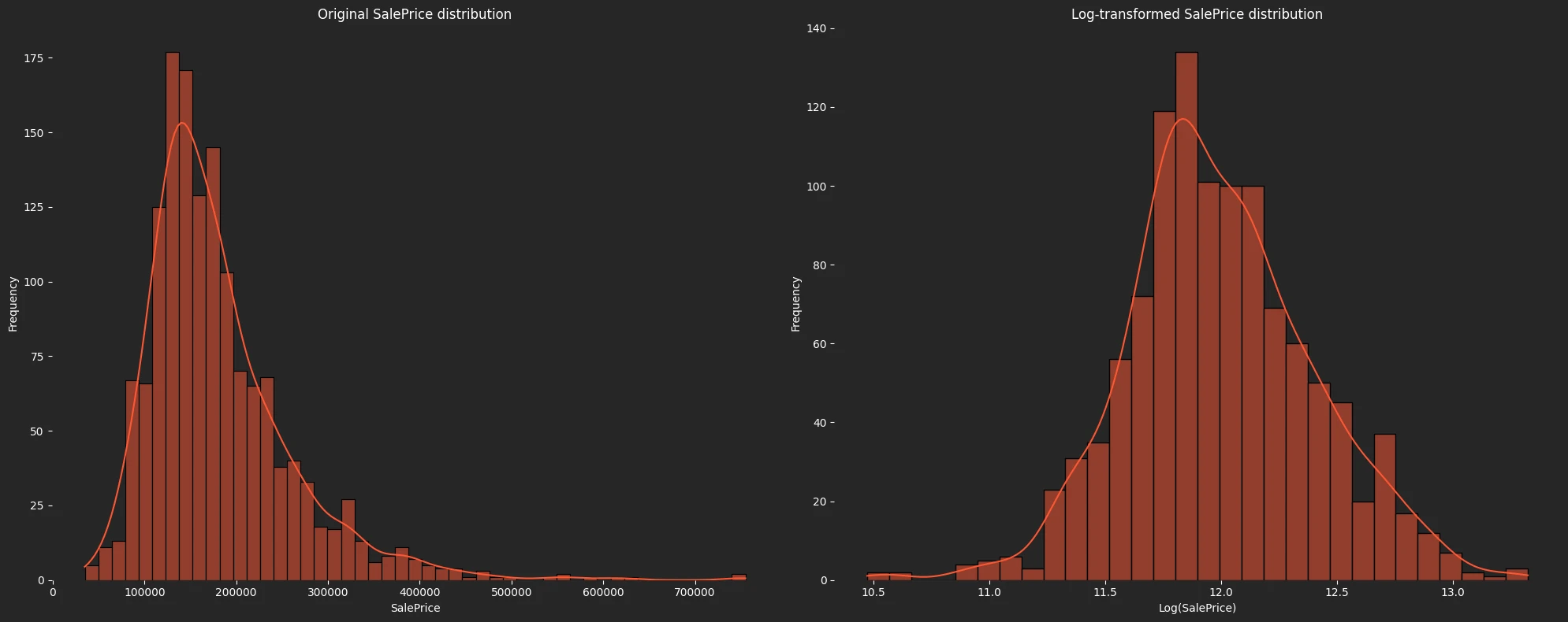
7. Log Transformation of SalePrice
8. Encoding of Columns
- Ordinal Features: Encoded using an ordinal encoder for ordered categories.
- Nominal Features: Encoded using one-hot encoding for unordered categories.
- Numerical Features: Imputed missing values and scaled for consistency.
# Define ordinal and nominal features
ode_cols = ['LotShape', 'LandContour', 'Utilities', 'LandSlope', 'BsmtQual',
            'BsmtFinType1', 'CentralAir', 'Functional', 'PoolQC', 'Fence',
            'FireplaceQu', 'GarageFinish', 'GarageQual', 'PavedDrive',
            'ExterCond', 'KitchenQual', 'BsmtExposure', 'HeatingQC',
            'ExterQual', 'BsmtCond']
ohe_cols = [col for col in train_df_log_transformed.select_dtypes(include=['object']).columns if col not in ode_cols]
num_cols = numeric_cols.drop('SalePrice')

# Define pipelines
ode_pipeline = Pipeline(steps=[
    ('impute', SimpleImputer(strategy='most_frequent')),
    ('ode', OrdinalEncoder(handle_unknown='use_encoded_value', unknown_value=-1))
])
ohe_pipeline = Pipeline(steps=[
    ('impute', SimpleImputer(strategy='most_frequent')),
    ('ohe', OneHotEncoder(handle_unknown='ignore', sparse_output=False))
])
num_pipeline = Pipeline(steps=[
    ('impute', SimpleImputer(strategy='mean')),
    ('scaler', StandardScaler())
])

# Build column transformer
col_trans = ColumnTransformer(transformers=[
    ('num_p', num_pipeline, num_cols),
    ('ode_p', ode_pipeline, ode_cols),
    ('ohe_p', ohe_pipeline, ohe_cols),
], remainder='passthrough', n_jobs=-1)9. Model Training
- Hyperparameter Tuning: Conducted a grid search using GridSearchCV to find the optimal hyperparameters for each model. This step involved cross-validation to minimize overfitting and ensure robust performance.
- Best Parameters: Extracted the best parameters for each model after grid search, such as the number of estimators, learning rate, or maximum depth.
- Final Training: Trained the models with the best parameters on the entire training dataset.
- Performance Metrics: Evaluated the models using Root Mean Squared Error (RMSE), a key metric for this competition.
- Random Forest Regressor (RFR): RMSE: 0.1393 | Best Parameters: max_depth=15, min_samples_split=3, n_estimators=250
- XGBoost (XGB): RMSE: 0.1252 | Best Parameters: learning_rate=0.05, max_depth=3, n_estimators=300
- Ridge Regression: RMSE: 0.1223 | Best Parameters: alpha=10, solver='sag'
- LightGBM (LGBM): RMSE: 0.1344 | Best Parameters: boosting_type='gbdt', learning_rate=0.05, n_estimators=200, num_leaves=20
- CatBoost (CB): RMSE: 0.1260 | Best Parameters: depth=5, iterations=500, learning_rate=0.05
10. Voting and Stacking
- Voting Regressor: Combined predictions from five models (Random Forest, XGBoost, Ridge Regression, LightGBM, and CatBoost) using equal weights. This approach leverages the strengths of individual models to produce a more robust prediction.
- Stacking Regressor: Used the predictions from the same five models as inputs to a final estimator (the Voting Regressor). This hierarchical ensemble technique captures complex relationships between base models, improving predictive accuracy.
- Voting Regressor: RMSE: 0.1009
- Stacking Regressor: RMSE: 0.1025