1. Introduction
2. Data Preparation
# Loading Data
train = pd.read_csv('../data/external/train.csv')
test = pd.read_csv('../data/external/test.csv')

# Separating Features and Labels
X = train.drop("label", axis=1)
y = train["label"]

# Data Normalization
X = X / 255.0
# Applying transformations to test.csv
X_test = test / 255.0

# Splitting Data into Training and Validation Sets
X_train, X_val, y_train, y_val = train_test_split(X, y, test_size=0.1, random_state=1)

# Preview Images
X_reshaped = X_train.to_numpy().reshape(-1, 28, 28, 1)
plt.figure(figsize=(15, 5))
for i in range(30):
    plt.subplot(3, 10, i+1)
    plt.imshow(X_reshaped[i, :, :, 0], cmap=plt.cm.binary)
    plt.axis('off')
plt.subplots_adjust(wspace=-0.1, hspace=-0.1)
plt.show()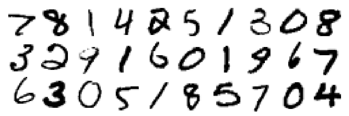
3. Dense Neural Network
- Layer 1 and 2: Use ReLU (Rectified Linear Unit) activation to capture complex patterns and avoid vanishing gradients.
- Layer 3: Uses softmax activation to output probabilities for each digit (0-9), ensuring outputs sum to 1 for multi-class classification.
# Defining the Model Architecture
model = Sequential([
    Dense(units=25, activation='relu'),
    Dense(units=15, activation='relu'),
    Dense(units=10, activation='softmax')
])

# Compiling the Model
model.compile(
    optimizer=Adam(learning_rate=1e-3),
    loss=SparseCategoricalCrossentropy(),
    metrics=['accuracy']
)

# Training the Model
model.fit(X_train, y_train, epochs=30, validation_data=(X_val, y_val))Epoch 1/30
1182/1182 ━━━━━━━━━━━━━━━━━━━━ 1s 1ms/step - accuracy: 0.9917 - loss: 0.0269 - val_accuracy: 0.9521 - val_loss: 0.2329
Epoch 2/30
1182/1182 ━━━━━━━━━━━━━━━━━━━━ 1s 1ms/step - accuracy: 0.9922 - loss: 0.0241 - val_accuracy: 0.9474 - val_loss: 0.2693
Epoch 3/30
1182/1182 ━━━━━━━━━━━━━━━━━━━━ 1s 1ms/step - accuracy: 0.9919 - loss: 0.0264 - val_accuracy: 0.9521 - val_loss: 0.25384. Understanding L2 Regularization
# Defining a Model with L2 Regularization
model = Sequential([
    Dense(units=25, activation='relu', kernel_regularizer=L2(0.001)),
    Dense(units=15, activation='relu', kernel_regularizer=L2(0.001)),
    Dense(units=10, activation='softmax', kernel_regularizer=L2(0.001))
])

# Compiling and Training the Model
model.compile(
    optimizer=Adam(learning_rate=1e-3),
    loss=SparseCategoricalCrossentropy(),
    metrics=['accuracy']
)
model.fit(X_train, y_train, epochs=30, validation_data=(X_val, y_val))Epoch 1/30
1182/1182 ━━━━━━━━━━━━━━━━━━━━ 3s 1ms/step - accuracy: 0.7596 - loss: 0.8735 - val_accuracy: 0.9155 - val_loss: 0.3734
Epoch 2/30
1182/1182 ━━━━━━━━━━━━━━━━━━━━ 1s 1ms/step - accuracy: 0.9291 - loss: 0.3518 - val_accuracy: 0.9388 - val_loss: 0.3181
Epoch 3/30
1182/1182 ━━━━━━━━━━━━━━━━━━━━ 1s 1ms/step - accuracy: 0.9393 - loss: 0.3115 - val_accuracy: 0.9414 - val_loss: 0.30265. Defining a Deeper, More Complex Model
# Defining the Model
model = Sequential([
    Dense(units=512, activation='relu', kernel_regularizer=L2(0.001)),  # Increased units
    Dropout(0.4),  # Add dropout to prevent overfitting
    Dense(units=256, activation='relu', kernel_regularizer=L2(0.001)),
    Dropout(0.4),
    Dense(units=128, activation='relu', kernel_regularizer=L2(0.001)),
    Dropout(0.3),
    Dense(units=64, activation='relu', kernel_regularizer=L2(0.001)),
    Dropout(0.3),
    Dense(units=32, activation='relu', kernel_regularizer=L2(0.001)),
    Dense(units=10, activation='softmax', kernel_regularizer=L2(0.001))
])

# Compiling and Training the Model
model.compile(
    optimizer=Adam(learning_rate=5e-5),  # Reduced learning rate for better convergence
    loss=SparseCategoricalCrossentropy(),
    metrics=['accuracy']
)
model.fit(X_train, y_train, epochs=50, validation_data=(X_val, y_val))Epoch 1/50
1182/1182 ━━━━━━━━━━━━━━━━━━━━ 8s 5ms/step - accuracy: 0.2657 - loss: 3.1987 - val_accuracy: 0.8098 - val_loss: 1.6949
Epoch 2/50
1182/1182 ━━━━━━━━━━━━━━━━━━━━ 5s 4ms/step - accuracy: 0.6886 - loss: 1.8662 - val_accuracy: 0.8867 - val_loss: 1.2846
Epoch 3/50
1182/1182 ━━━━━━━━━━━━━━━━━━━━ 6s 5ms/step - accuracy: 0.8061 - loss: 1.4826 - val_accuracy: 0.9083 - val_loss: 1.1397
# Truncated for brevity...
Epoch 50/50
1182/1182 ━━━━━━━━━━━━━━━━━━━━ 5s 4ms/step - accuracy: 0.9839 - loss: 0.2517 - val_accuracy: 0.9802 - val_loss: 0.26696. Convolutional Neural Network (CNN)
# Reshape the Data
X_train = X_train.to_numpy().reshape(-1, 28, 28, 1)
X_val = X_val.to_numpy().reshape(-1, 28, 28, 1)
X_test = X_test.to_numpy().reshape(-1, 28, 28, 1)# CNN Model
model = Sequential([
Conv2D(32, kernel_size=(3, 3), activation='relu', padding='Same',
kernel_regularizer=L2(0.0001), input_shape=(28, 28, 1)),
MaxPooling2D(pool_size=(2, 2)),
Dropout(0.2),
Conv2D(64, kernel_size=(3, 3), activation='relu', padding='Same',
kernel_regularizer=L2(0.0001)),
MaxPooling2D(pool_size=(2, 2)),
Dropout(0.3),
Conv2D(128, kernel_size=(3, 3), activation='relu', padding='Same',
kernel_regularizer=L2(0.0001)),
MaxPooling2D(pool_size=(2, 2)),
Dropout(0.3),
Flatten(),
Dense(64, activation='relu', kernel_regularizer=L2(0.0001)),
Dropout(0.2),
Dense(10, activation='softmax')
])model.compile(
optimizer=Adam(learning_rate=1e-4),
loss=SparseCategoricalCrossentropy(),
metrics=['accuracy']
)
model.fit(X_train, y_train, epochs=50, validation_data=(X_val, y_val))Epoch 1/50
1182/1182 ━━━━━━━━━━━━━━━━━━━━ 13s 9ms/step - accuracy: 0.4787 - loss: 1.5297 - val_accuracy: 0.9433 - val_loss: 0.2257
Epoch 2/50
1182/1182 ━━━━━━━━━━━━━━━━━━━━ 11s 10ms/step - accuracy: 0.9082 - loss: 0.3163 - val_accuracy: 0.9626 - val_loss: 0.1593
...
Epoch 49/50
1182/1182 ━━━━━━━━━━━━━━━━━━━━ 12s 11ms/step - accuracy: 0.9921 - loss: 0.0510 - val_accuracy: 0.9933 - val_loss: 0.0500
Epoch 50/50
1182/1182 ━━━━━━━━━━━━━━━━━━━━ 13s 11ms/step - accuracy: 0.9925 - loss: 0.0500 - val_accuracy: 0.9912 - val_loss: 0.05117. Data Augmentation
# Data Augmentation
datagen = ImageDataGenerator(
    rotation_range=5,
    zoom_range=0.1,
    width_shift_range=0.1,
    height_shift_range=0.1
)
datagen.fit(X_train)# CNN with Batch Normalization
model = Sequential([
Conv2D(64, kernel_size=(3, 3), activation='relu', padding='Same',
kernel_regularizer=L2(0.0001), input_shape=(28, 28, 1)),
BatchNormalization(),
MaxPooling2D(pool_size=(2, 2)),
Dropout(0.3),
Conv2D(128, kernel_size=(3, 3), activation='relu', padding='Same',
kernel_regularizer=L2(0.0001)),
BatchNormalization(),
MaxPooling2D(pool_size=(2, 2)),
Dropout(0.3),
Conv2D(256, kernel_size=(3, 3), activation='relu', padding='Same',
kernel_regularizer=L2(0.0001)),
BatchNormalization(),
MaxPooling2D(pool_size=(2, 2)),
Dropout(0.4),
Flatten(),
Dense(128, activation='relu', kernel_regularizer=L2(0.0001)),
Dropout(0.4),
Dense(64, activation='relu', kernel_regularizer=L2(0.0001)),
Dropout(0.3),
Dense(10, activation='softmax')
])Epoch 1/50
1182/1182 ━━━━━━━━━━━━━━━━━━━━ 55s 44ms/step - accuracy: 0.2394 - loss: 2.3610 - val_accuracy: 0.9124 - val_loss: 0.4081
Epoch 2/50
1182/1182 ━━━━━━━━━━━━━━━━━━━━ 55s 47ms/step - accuracy: 0.7042 - loss: 0.9476 - val_accuracy: 0.9610 - val_loss: 0.1870
...
Epoch 49/50
1182/1182 ━━━━━━━━━━━━━━━━━━━━ 62s 52ms/step - accuracy: 0.9887 - loss: 0.0851 - val_accuracy: 0.9955 - val_loss: 0.0688
Epoch 50/50
1182/1182 ━━━━━━━━━━━━━━━━━━━━ 65s 55ms/step - accuracy: 0.9888 - loss: 0.0902 - val_accuracy: 0.9943 - val_loss: 0.07018. Model Evaluation
# Plot Training vs Validation Accuracy
fig, ax = plt.subplots()
fig.patch.set_facecolor(CFG.background_color)
ax.set_facecolor(CFG.background_color)
ax.plot(history.history['accuracy'], label='train accuracy', color=CFG.point_color)
ax.plot(history.history['val_accuracy'], label='validation accuracy', color='skyblue')
legend = ax.legend(facecolor=CFG.background_color, edgecolor=CFG.font_color)
plt.setp(legend.get_texts(), color=CFG.font_color)
ax.set_title("Training vs Validation Accuracy", color=CFG.font_color)
ax.set_xlabel("Epoch", color=CFG.font_color)
ax.set_ylabel("Accuracy", color=CFG.font_color)
ax.tick_params(colors=CFG.font_color)
for spine in ax.spines.values():
    spine.set_visible(False)
plt.show()

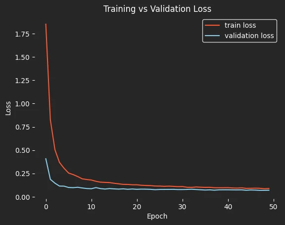
# Plot Training vs Validation Loss
fig, ax = plt.subplots()
fig.patch.set_facecolor(CFG.background_color)
ax.set_facecolor(CFG.background_color)
ax.plot(history.history['loss'], label='train loss', color=CFG.point_color)
ax.plot(history.history['val_loss'], label='validation loss', color='skyblue')
legend = ax.legend(facecolor=CFG.background_color, edgecolor=CFG.font_color)
plt.setp(legend.get_texts(), color=CFG.font_color)
ax.set_title("Training vs Validation Loss", color=CFG.font_color)
ax.set_xlabel("Epoch", color=CFG.font_color)
ax.set_ylabel("Loss", color=CFG.font_color)
ax.tick_params(colors=CFG.font_color)
for spine in ax.spines.values():
    spine.set_visible(False)
plt.show()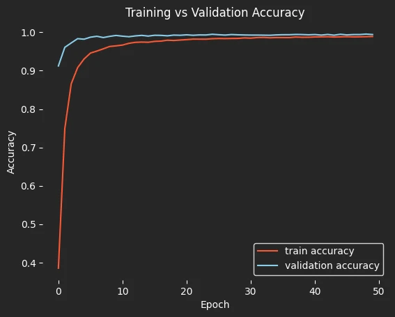
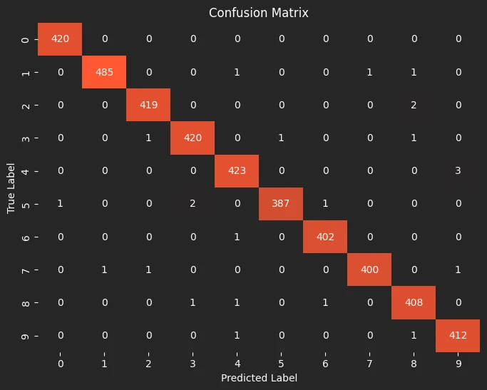
# Generate Confusion Matrix
y_pred_probs = model.predict(X_val)  # Predict probabilities
y_pred = np.argmax(y_pred_probs, axis=1)  # Convert probabilities to class labels

# Create confusion matrix
conf_matrix = confusion_matrix(y_val, y_pred)
class_names = [i for i in range(10)]

# Plot the confusion matrix
custom_cmap = LinearSegmentedColormap.from_list([CFG.background_color, CFG.point_color])
fig, ax = plt.subplots(figsize=(8, 6))
fig.patch.set_facecolor(CFG.background_color)
ax.set_facecolor(CFG.background_color)
sns.heatmap(conf_matrix, annot=True, fmt='d', cmap=custom_cmap, xticklabels=class_names,
            yticklabels=class_names, cbar=False, annot_kws={"color": CFG.font_color})
ax.set_xlabel('Predicted Label', color=CFG.font_color)
ax.set_ylabel('True Label', color=CFG.font_color)
ax.set_title('Confusion Matrix', color=CFG.font_color)
ax.tick_params(axis='x', colors=CFG.font_color)
ax.tick_params(axis='y', colors=CFG.font_color)
for spine in ax.spines.values():
    spine.set_visible(False)
plt.show()